|
Size: 4707
Comment:
|
Size: 4708
Comment:
|
| Deletions are marked like this. | Additions are marked like this. |
| Line 53: | Line 53: |
| * Please not that high-pass filter is applied at the frequency specified by fcut. This is needed to minimize the FIR filter length to get reasonable computation time | * Please note that high-pass filter is applied at the frequency specified by fcut. This is needed to minimize the FIR filter length to get reasonable computation time |
Step 6: Make FIR filters and save into a npz file
- We assume a simple DARM model with
- Actuation (A) with f^{-2} (fc=0.7, Q=100) and delay of 61 us x2
- Sensing (C) with frequency independent and delay of 61 us
- Here is a small piece of python code to represent a f^{-2} pole
   1 # Convert f0 and Q to a pair of complex numbers
   2 def fq2c(f0, Q, rad=False):
   3     w0 = -f0 if rad else -2*np.pi*f0
   4     a  = w0/(2*Q)
   5     b  = w0/(2*Q)*np.sqrt(4*Q**2-1)
   6     return np.array([a+1j*b, a-1j*b])
   7
   8 # Complex-conjugate pair of poles at f with Q and the DC gain = gn
   9 def pole2(f, Q, gn=1, dt=0, rad=False):
  10     (a,b) = fq2c(f, Q, rad);
  11     w1 = 2j*np.pi
  12     g0 = abs(1/(w1-a)/(w1-b))
  13     return sg.lti([], [a,b], gn/g0, dt=dt)
- Here is the part to define DARM model parameters
   1 fNyq = 8192           # Nyquist frequency
   2
   3 # Actuation model
   4 f0   = 0.7            # pole frequency
   5 Q    = 100            # pole Q
   6 gn   = 0.917e-10      # actuation gain (m/ct)
   7 tda  = 2*(1./2)**14   # actuation delay (2 digits)
   8 Tla  = 2.             # Length of time-domain filter in second
   9 fca  = 4.             # High-pass filter frequency
  10 dla  = Tla*fNyq
  11 act  = pole2(f0, Q, gn)
  12
  13 # Inverse sensing model
  14 C    = 9.356e-12      # inverse optical gain (m/ct)
  15 tdc  = (1./2)**14     # sensing delay (1 digit)
  16 Tlc  = 0.5            # Length of time-domain filter in second
  17 fcc  = 8.             # High-pass filter frequency
  18 dlc  = Tlc*fNyq
  19 sen  = sg.lti([], [], C)
- Here is the part to generate the FIR filter and save to npz (numpy zipped) file
- Another python script gentd.py contains the actual part to generate time-domain FIR filter
- Here is a core part of gentd.py. It is just an inverse-FFT from frequency response data into time domain
- Please note that high-pass filter is applied at the frequency specified by fcut. This is needed to minimize the FIR filter length to get reasonable computation time
   1 # Generate time domain FIR filter of LTI system
   2 def gentd(sys, td=0, fcut=4, Tl=2, fNyq=8192):
   3 ...
   4     # Apply Hann window to roll off low frequencies
   5     h[0:2*hp] = h[0:2*hp]*cond[0:2*hp]
   6
   7     h[0]    = 0   # Zero out the DC component
   8     h[Nf-1] = 0   # Zero out the Nyquist component
   9
  10     # Apply delay
  11     delay = np.exp(-1j*w*(np.floor(Tl*fNyq)*dt+td))
  12     h     = h*delay
  13
  14     # Fill out negative frequencies
  15     for k in np.arange(0, Nf-2):
  16         h = np.append(h, np.conj(h[Nf-k-2]))
  17
  18     # Take inverse Fourier transform
  19     td = np.fft.ifft(h)
  20     td = td.real-td[0].real
- The python script is available at git repository
> kagra-cal/Observation/Phase1/tutorials/genfl
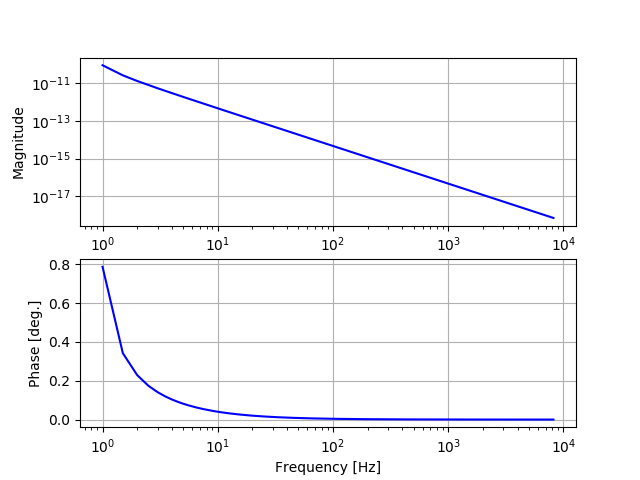
- The bode plot shows the the frequency response of the actuation filter
- Check the contents of the output file (filt.npz)
> python
>>> import numpy as np
>>> import matplotlib.pyplot as plt
>>> fig=plt.figure()
>>> fl=np.load('filt.npz')
>>> plt.plot(fl['a'])
>>> fig.show()
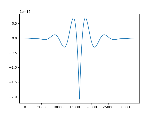
>>> plt.savefig('afilt.png')- The plot shows the time domain FIR coefficients (= impulse response) for the actuation filter


