|
Size: 1531
Comment:
|
Size: 2412
Comment:
|
| Deletions are marked like this. | Additions are marked like this. |
| Line 9: | Line 9: |
| the original data into some appropriate data sets that contributes to some frequency bands. Basically the EMD is described by a sifting function defined as {{https://upload.wikimedia.org/math/e/e/4/ee4471f673afaddfc791f692cf250f6b.png}}, which shows that the EMD performs the subtraction between the original data (or the previously generated data) and its average of envelopes, repeatedly, called '''''intrinsic mode functions (IMF)''''', expressed by {{https://upload.wikimedia.org/math/7/e/c/7ec2bae54bcdd79fab725ef8d6c5314c.png}} and {{https://upload.wikimedia.org/math/6/5/3/65349fc2c693c1b809562b59f4b5e172.png}}. The Hilbert transform of the ''EMDed data'' consists of the amplitude and phase parts and we see that the original data can be expressed by the summation of the whole IMFs, which is {{https://upload.wikimedia.org/math/9/d/e/9de1f9c2b24c4c2b3bab29243d825bc3.png}}. |
the original data into some appropriate data sets that contributes to some frequency bands. Basically the EMD is described by a sifting processes with {{https://upload.wikimedia.org/math/e/e/4/ee4471f673afaddfc791f692cf250f6b.png}}, which shows that the EMD performs the subtraction between the original data (or the previously generated data) and its average of envelopes, repeatedly, called '''''intrinsic mode functions (IMF)''''', expressed by {{https://upload.wikimedia.org/math/7/e/c/7ec2bae54bcdd79fab725ef8d6c5314c.png}} and {{https://upload.wikimedia.org/math/6/5/3/65349fc2c693c1b809562b59f4b5e172.png}}. The Hilbert transform of the ''EMDed data'' consists of the amplitude and phase parts and we see that the original data can be expressed by the summation of the whole IMFs, which is {{https://upload.wikimedia.org/math/6/f/d/6fdad0aefbac705612d1e8541fcd9eef.png}}. |
| Line 12: | Line 12: |
| Comparing to the (Fast) Fourier Transform (FFT), {{https://upload.wikimedia.org/math/2/7/7/277cc4bee5968c6ca2d4c78747d18689.png}}, we easily see that the HHT deals with the time-variant amplitude and phase data with adaptive bases. | |
| Line 13: | Line 14: |
| ||<bgcolor="#E0E0FF"> ||<bgcolor="#E0E0FF"> Fourier ||<bgcolor="#E0E0FF"> Wavelet ||<bgcolor="#E0E0FF"> Hilbert-Huang || ||<bgcolor="#E0E0FF">Basis || a priori || a priori || Adaptive || ||<bgcolor="#E0E0FF">Frequency || Integral transform: Global || Integral transform: Regional || Differentiation: Local|| ||<bgcolor="#E0E0FF">Presentation || Energy-Frequency || Energy-Time-Frequency || Energy-Time-Frequency|| ||<bgcolor="#E0E0FF"> Nonlinearity || No || No || Yes || ||<bgcolor="#E0E0FF"> Non-stationarity || No || Yes || Yes || ||<bgcolor="#E0E0FF"> Uncertainty || Yes || Yes || No || ||<bgcolor="#E0E0FF">Harmonics || Yes || Yes || No || |
HHT based Instrumental Glitch Trigger Generation
Project Description
- Introduction: Hilbert-Huang Transform (HHT)
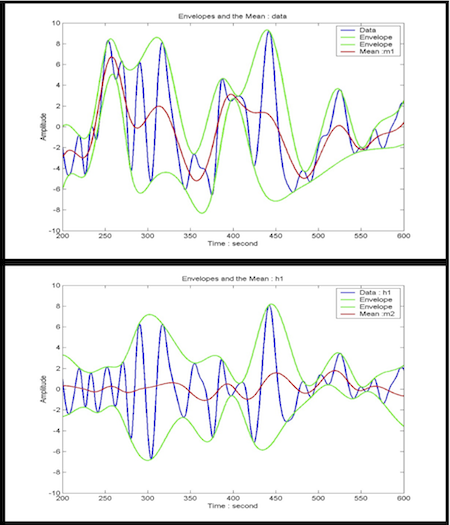
 HHT is a recently suggested empirical data transform based on adaptive bases. So it is very useful for analyzing non-linear and/or non-stationary data. The HHT consists of two main parts: 1) empirical mode decomposition (EMD) 2) Hilbert transform. The EMD can decompose the original data into some appropriate data sets that contributes to some frequency bands. Basically the EMD is described by a sifting processes with
  , which shows that the EMD performs the subtraction between the original data (or the previously generated data) and its average of envelopes, repeatedly, called intrinsic mode functions (IMF), expressed by
  and
and  . The Hilbert transform of the EMDed data consists of the amplitude and phase parts and we see that the original data can be expressed by the summation of the whole IMFs, which is
  .
.
Comparing to the (Fast) Fourier Transform (FFT),  , we easily see that the HHT deals with the time-variant amplitude and phase data with adaptive bases.
|
Fourier |
Wavelet |
Hilbert-Huang |
Basis |
a priori |
a priori |
Adaptive |
Frequency |
Integral transform: Global |
Integral transform: Regional |
Differentiation: Local |
Presentation |
Energy-Frequency |
Energy-Time-Frequency |
Energy-Time-Frequency |
Nonlinearity |
No |
No |
Yes |
Non-stationarity |
No |
Yes |
Yes |
Uncertainty |
Yes |
Yes |
No |
Harmonics |
Yes |
Yes |
No |
Goal
Preliminary Analysis of HHT
Trigger Generation Method
Simulation Results
