|
Size: 771
Comment:
|
Size: 7433
Comment:
|
| Deletions are marked like this. | Additions are marked like this. |
| Line 2: | Line 2: |
| ==== Project Description ==== * Introduction: Hilbert-Huang Transform (HHT) HHT is a recently suggested empirical data transform based on adaptive bases. So it is very useful for analyzing non-linear and/or non-stationary data. The HHT consists of two main parts: 1) empirical mode decomposition (EMD) 2) Hilbert transform. The EMD can decompose the original data into some appropriate data sets that contributes to some frequency bands. Basically the EMD is described by a sifting function defined as {{CodeCogsEqn.png}} ==== Goal ==== |
==== Project Description and Goal ==== * Member: John J. Oh, Sang Hoon Oh, Edwin J. Son (NIMS), Young-Min Kim (Pusan National Univ.), Kazuhiro Hayama (Osaka Univ.) * Used Data: S6 Auxiliary Channel Data, KAGRA Seismic/Magnetometer Data * Goal: Developing an improved trigger generation scheme using HHT - comparing KW triggers (and others) ==== Introduction: Hilbert-Huang Transform (HHT) ==== {{attachment:emds.png||align="left"}} HHT is a recently suggested empirical data transform based on adaptive bases. So it is very useful for analyzing non-linear and/or non-stationary data. The HHT consists of two main parts: 1) empirical mode decomposition (EMD) 2) Hilbert spectral analysis (HSA). The EMD can decompose the original data into some appropriate data sets that contributes to some frequency bands. Basically the EMD is described by a sifting processes with {{https://upload.wikimedia.org/math/e/e/4/ee4471f673afaddfc791f692cf250f6b.png}}, which shows that the EMD performs the subtraction between the original data (or the previously generated data) and its average of envelopes, repeatedly, called '''''intrinsic mode functions (IMF)''''', expressed by {{https://upload.wikimedia.org/math/7/e/c/7ec2bae54bcdd79fab725ef8d6c5314c.png}} and {{https://upload.wikimedia.org/math/6/5/3/65349fc2c693c1b809562b59f4b5e172.png}}. And the normalized squared difference (NSD) between two successive sifting operations is defined as {{https://upload.wikimedia.org/math/1/8/a/18aba9375519cd1b75a761363eea55b7.png}}, which should be small. The stoppage criterion of this process is determined by comparing between the NSD and the predetermined value - if NSD is smaller than a predetermined value, the process is stopped. The Hilbert transform of the ''EMDed data'' consists of the amplitude and phase parts and we see that the original data can be expressed by the summation of the whole IMFs, which is {{https://upload.wikimedia.org/math/6/f/d/6fdad0aefbac705612d1e8541fcd9eef.png}}. Comparing to the (Fast) Fourier Transform (FFT), {{https://upload.wikimedia.org/math/2/7/7/277cc4bee5968c6ca2d4c78747d18689.png}}, we easily see that the HHT deals with the time-variant amplitude and phase data with adaptive bases. We compare the HHT to other two different transforms in the following table. ||<bgcolor="#E0E0FF"> ||<style="text-align: center;background-color: #E0E0FF;"> Fourier ||<style="text-align: center;background-color: #E0E0FF;"> Wavelet ||<style="text-align: center;background-color: #E0E0FF;"> Hilbert-Huang || ||<style="text-align: center;background-color: #E0E0FF;"> Basis ||<style="text-align: center;"> a priori ||<style="text-align: center;"> a priori ||<style="text-align: center;"> Adaptive || ||<style="text-align: center;background-color: #E0E0FF;"> Frequency ||<style="text-align: center;"> Integral transform: Global ||<style="text-align: center;"> Integral transform: Regional ||<style="text-align: center;"> Differentiation: Local || ||<style="text-align: center;background-color: #E0E0FF;"> Presentation ||<style="text-align: center;"> Energy-Frequency ||<style="text-align: center;"> Energy-Time-Frequency ||<style="text-align: center;"> Energy-Time-Frequency || ||<style="text-align: center;background-color: #E0E0FF;"> Nonlinearity ||<style="text-align: center;"> No ||<style="text-align: center;"> No ||<style="text-align: center;"> Yes || ||<style="text-align: center;background-color: #E0E0FF;"> Non-stationarity ||<style="text-align: center;"> No ||<style="text-align: center;"> Yes ||<style="text-align: center;"> Yes || ||<style="text-align: center;background-color: #E0E0FF;"> Uncertainty ||<style="text-align: center;"> Yes ||<style="text-align: center;"> Yes ||<style="text-align: center;"> No || ||<style="text-align: center;background-color: #E0E0FF;"> Harmonics ||<style="text-align: center;"> Yes ||<style="text-align: center;"> Yes ||<style="text-align: center;"> No || |
| Line 9: | Line 30: |
| Here, we show some preliminary results done so far using HHT with S6 LIGO data and KAGRA data. First we ran HHT code written in python - mainly consists of EMD and HSA parts with auxiliary channel data in LIGO S6, for example, L1_SUS_ITMX_OPLEV_Y and L1_LSC_DARM_ERR. We ran the code for so many data sets but here some of them are presented to explain our motivation. * Trigger Generation Criterion (Should be tuned later) * ''Ref.) Li Ming-Ai, Yang Lin-Bao, and Yang Jin-Fu, Commun. Info. Sci. Mag. Eng., Vol.1, No.2, PP.1-6 (2011)'' * When amplitude exceeds the threshold: {{https://upload.wikimedia.org/math/4/6/1/4616be59479f5b391affa35f797f5ea4.png}} then a trigger candidate is reported, where {{https://upload.wikimedia.org/math/1/e/b/1ebfaa5206b1858adef8686594c98da2.png}}. Note that A is an amplitude in a given segment, j is an index of IMFs, M denotes a mean value of the amplitude, X denotes peaks of amplitude, and s is an index of threshold. * HHT-based Trigger Check with S6 LIGO Data * Data: L1_SUS_ITMX_OPLEV_Y / L1_LSC-DARM_ERR * Method: HHT operation / KW Trigger at given GPS time * EMD Decomposition and HSA Trigger Generation / Comparison with KW Trigger (red) * The first thing is to compare the result done by HHT with the KW trigger as confirmed as an instrumental glitch (red in the figure). * For the KW trigger at a given GPS time, HHT can find the same trigger. * In IMF1 figure (Aux), HHT can also find very small glitch-like peaks (at 0.8, 1.8, and 2.7 GPU time) * In IMF5 figure (DARM), HHT finds the same glitch found in the KW transform at around 3.0 as well as so many glitch candidates before and after the red event time. {{attachment:S6HHT_KW.png|alt Comparison btw HHT & KW triggers of S6 aux. channel Data |width=800 height=250}} * Data: S6_968654557 (Big Dog Event) * Method: HHT operation / Big Dog time (around 8 sec in IMF3) * EMD Decomposition and HSA Trigger Generation (green) * To find the characteristic of HHT, we ran the code for the famous Big Dog Event (h of t data: obtained in the LIGO website). * The Big Dog Event lasts around 5 seconds in different frequency bands (starts from 30Hz to 100Hz) * In IMF3, the strongest peak at right before 8 second can be detected while other small trigger candidates can be found by our trigger generation scheme. * In IMF6, there are one trigger candidate at around 7 sec. * In conclusion, all these candidates could be GW signal or instrumental glitches. However the conclusion is that we can find some abnormal features of data in individually decomposed modes generated by HHT. {{attachment:S6HHT_BigDog.png|alt Big Dog Trigger seen in HHT |width=800 height=250}} * HHT-based Trigger Check with KAGRA Data * Data: 20131023_SEISMIC_SEI_NS_00000-00128 * Method: HHT operation * EMD Decompostion / HSA - marking in GPS time (green) {{attachment:20131023_seismic_SEI_NS_00000-00128_emd_0.png|alt HHT Triggers of KAGRA Seismic Data |width=850 height=250}} * Power Spectrum Density (Energy-Frequency Map) {{attachment:20131023_seismic_SEI_NS_00000-00128_psd.png|alt PSD of KAGRA Seismic Data |width=850 height=250}} |
HHT based Instrumental Glitch Trigger Generation
Project Description and Goal
- Member: John J. Oh, Sang Hoon Oh, Edwin J. Son (NIMS), Young-Min Kim (Pusan National Univ.), Kazuhiro Hayama (Osaka Univ.)
- Used Data: S6 Auxiliary Channel Data, KAGRA Seismic/Magnetometer Data
- Goal: Developing an improved trigger generation scheme using HHT - comparing KW triggers (and others)
Introduction: Hilbert-Huang Transform (HHT)
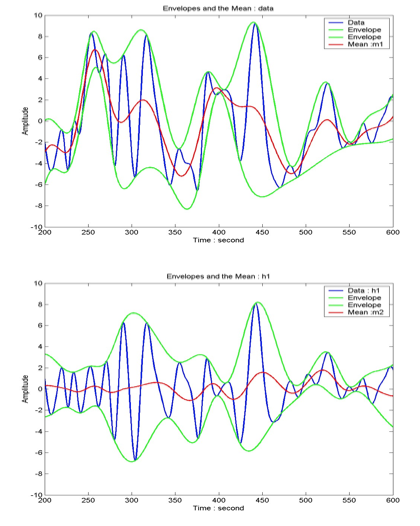
HHT is a recently suggested empirical data transform based on adaptive bases. So it is very useful for analyzing non-linear and/or non-stationary data. The HHT consists of two main parts: 1) empirical mode decomposition (EMD) 2) Hilbert spectral analysis (HSA). The EMD can decompose the original data into some appropriate data sets that contributes to some frequency bands. Basically the EMD is described by a sifting processes with
 , which shows that the EMD performs the subtraction between the original data (or the previously generated data) and its average of envelopes, repeatedly, called intrinsic mode functions (IMF), expressed by
  and
and  . And the normalized squared difference (NSD) between two successive sifting operations is defined as
 ,
,
which should be small. The stoppage criterion of this process is determined by comparing between the NSD and the predetermined value - if NSD is smaller than a predetermined value, the process is stopped.
The Hilbert transform of the EMDed data consists of the amplitude and phase parts and we see that the original data can be expressed by the summation of the whole IMFs, which is
 .
. Comparing to the (Fast) Fourier Transform (FFT),
 , we easily see that the HHT deals with the time-variant amplitude and phase data with adaptive bases. We compare the HHT to other two different transforms in the following table.
|
Fourier |
Wavelet |
Hilbert-Huang |
Basis |
a priori |
a priori |
Adaptive |
Frequency |
Integral transform: Global |
Integral transform: Regional |
Differentiation: Local |
Presentation |
Energy-Frequency |
Energy-Time-Frequency |
Energy-Time-Frequency |
Nonlinearity |
No |
No |
Yes |
Non-stationarity |
No |
Yes |
Yes |
Uncertainty |
Yes |
Yes |
No |
Harmonics |
Yes |
Yes |
No |
Preliminary Analysis of HHT
Here, we show some preliminary results done so far using HHT with S6 LIGO data and KAGRA data. First we ran HHT code written in python - mainly consists of EMD and HSA parts with auxiliary channel data in LIGO S6, for example, L1_SUS_ITMX_OPLEV_Y and L1_LSC_DARM_ERR. We ran the code for so many data sets but here some of them are presented to explain our motivation.
- Trigger Generation Criterion (Should be tuned later)
Ref.) Li Ming-Ai, Yang Lin-Bao, and Yang Jin-Fu, Commun. Info. Sci. Mag. Eng., Vol.1, No.2, PP.1-6 (2011)
- When amplitude exceeds the threshold:
- then a trigger candidate is reported, where
 .
.
- HHT-based Trigger Check with S6 LIGO Data
- Data: L1_SUS_ITMX_OPLEV_Y / L1_LSC-DARM_ERR
- Method: HHT operation / KW Trigger at given GPS time
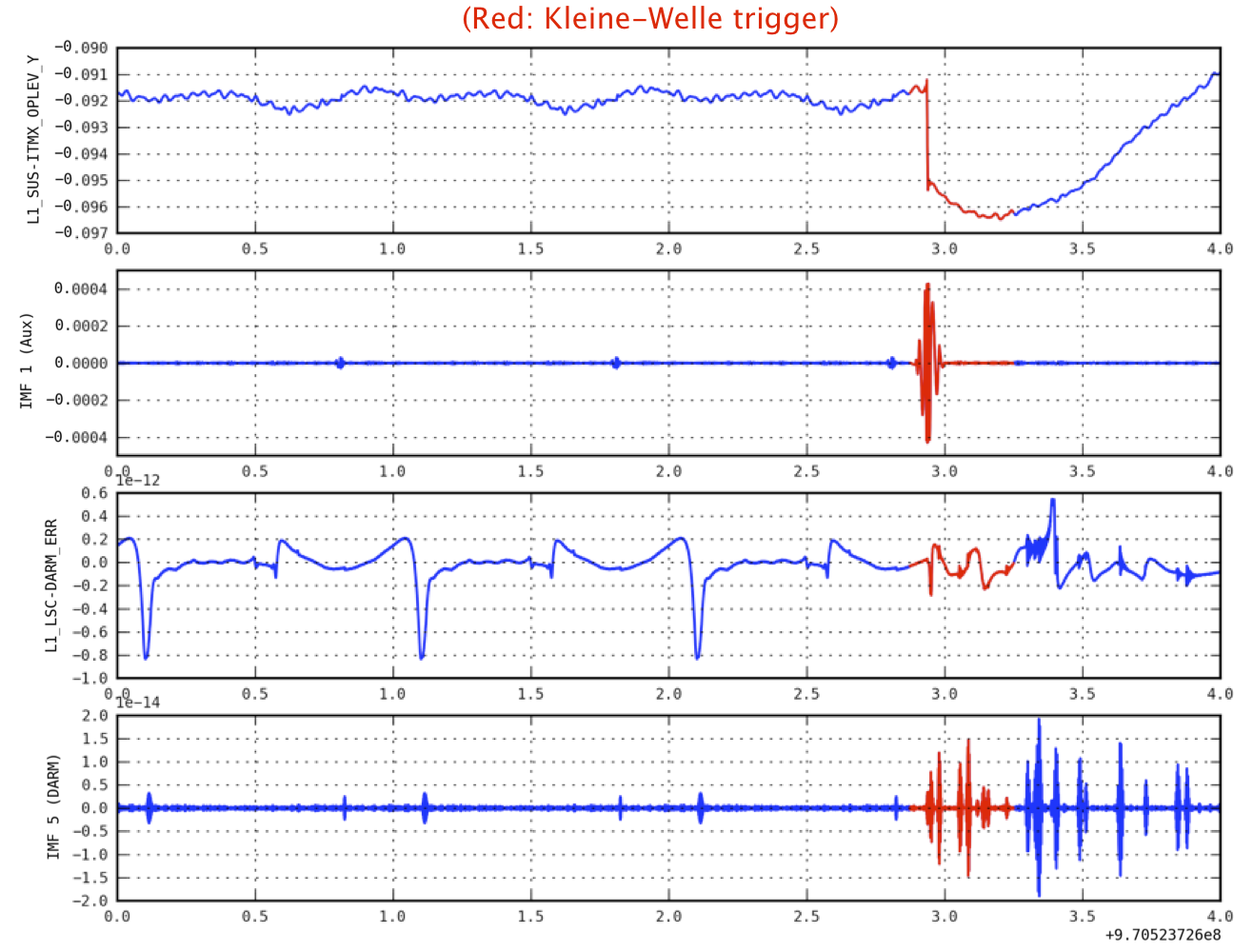
- EMD Decomposition and HSA Trigger Generation / Comparison with KW Trigger (red)
- The first thing is to compare the result done by HHT with the KW trigger as confirmed as an instrumental glitch (red in the figure).
- For the KW trigger at a given GPS time, HHT can find the same trigger.
- In IMF1 figure (Aux), HHT can also find very small glitch-like peaks (at 0.8, 1.8, and 2.7 GPU time)
- In IMF5 figure (DARM), HHT finds the same glitch found in the KW transform at around 3.0 as well as so many glitch candidates before and after the red event time.
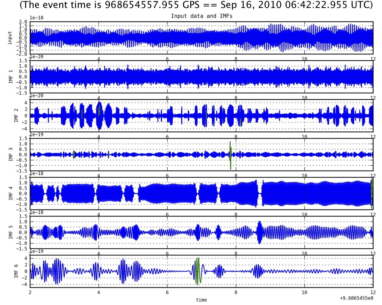
- Data: S6_968654557 (Big Dog Event)
- Method: HHT operation / Big Dog time (around 8 sec in IMF3)
- EMD Decomposition and HSA Trigger Generation (green)
- To find the characteristic of HHT, we ran the code for the famous Big Dog Event (h of t data: obtained in the LIGO website).
- The Big Dog Event lasts around 5 seconds in different frequency bands (starts from 30Hz to 100Hz)
- In IMF3, the strongest peak at right before 8 second can be detected while other small trigger candidates can be found by our trigger generation scheme.
- In IMF6, there are one trigger candidate at around 7 sec.
- In conclusion, all these candidates could be GW signal or instrumental glitches. However the conclusion is that we can find some abnormal features of data in individually decomposed modes generated by HHT.
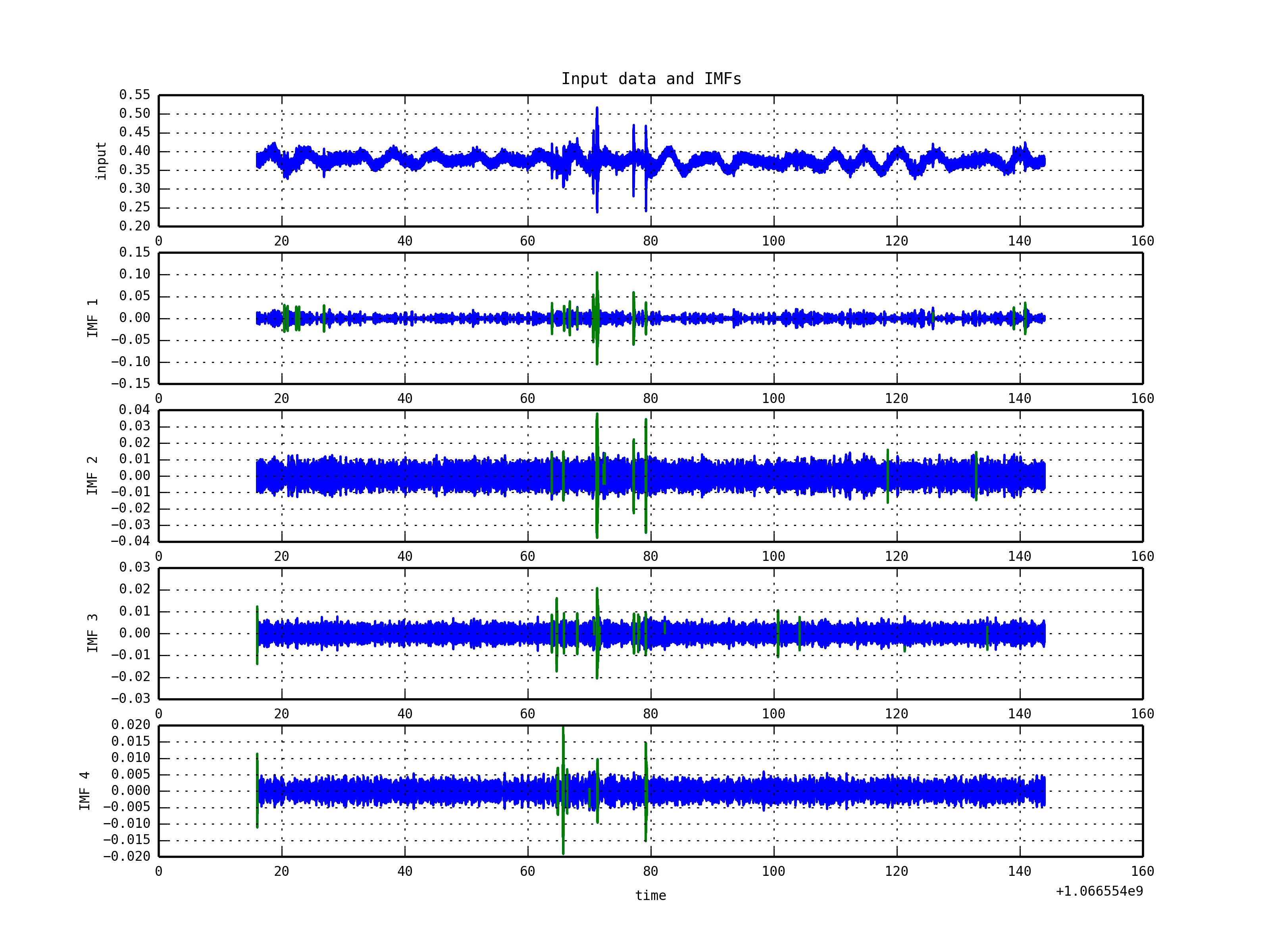
- HHT-based Trigger Check with KAGRA Data
- Data: 20131023_SEISMIC_SEI_NS_00000-00128
- Method: HHT operation
- EMD Decompostion / HSA - marking in GPS time (green)
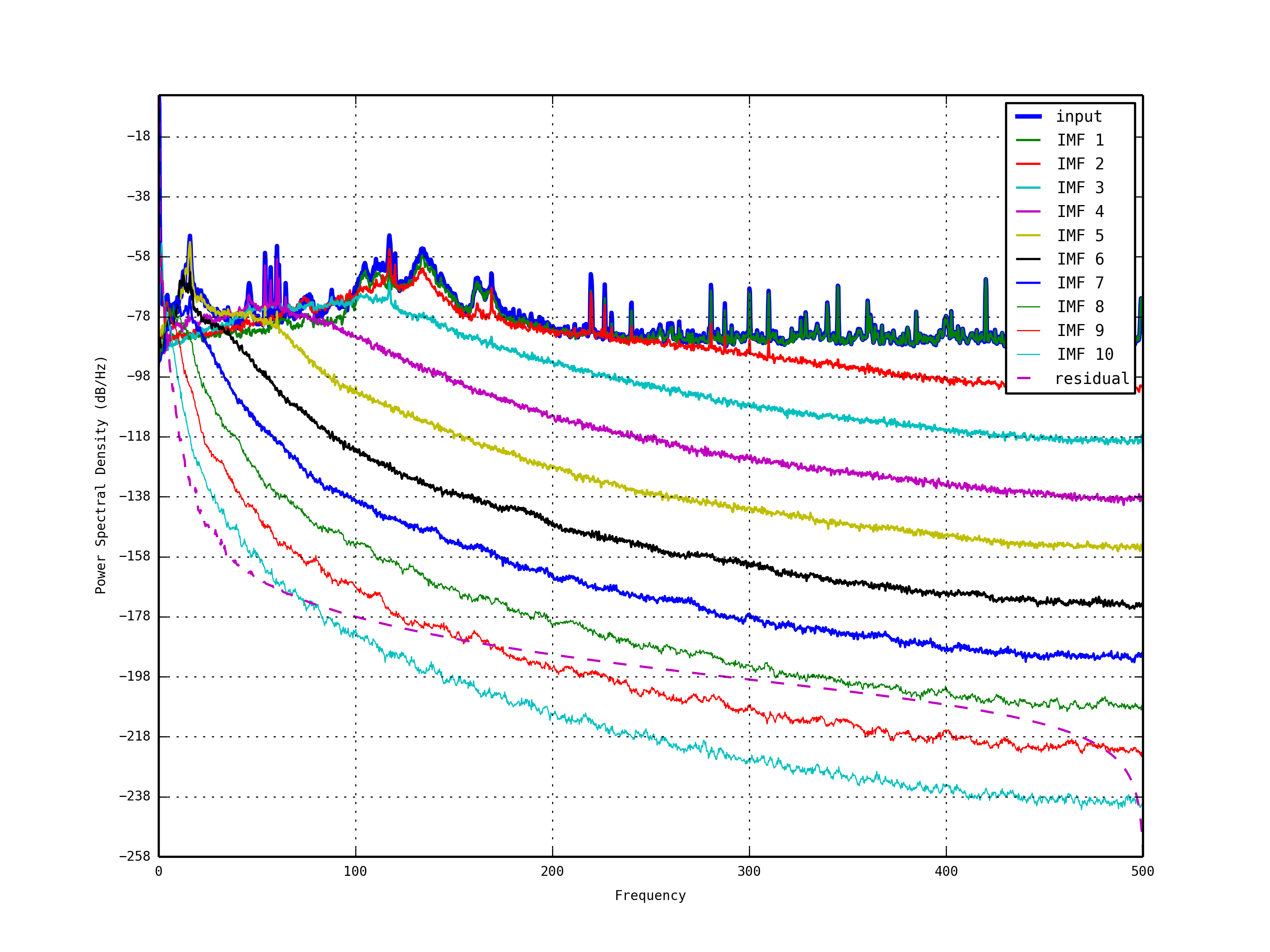
- Power Spectrum Density (Energy-Frequency Map)
Trigger Generation Method
Simulation Results


