This is the draft of the oplev diagonalization procedure.
Within the directory /kagra/Dropbox/Subsystems/VIS/TypeBData/oplev/measurements/ create a subdirectory according to the date and the suspension you are working with. For instance, if you arre working with SR2 on the 30th of March 2020 create the following directory: /kagra/Dropbox/Subsystems/VIS/TypeBData/oplev/measurements/SR2/20200330/.
Into the newly created directory copy the template xml files from /kagra/Dropbox/Subsystems/VIS/TypeBData/oplev/templates/. Copy the ones for the appropriate suspension.
From the directoty /kagra/Dropbox/Subsystems/VIS/TypeBData/oplev/templates/ copy the Matlab script oplev_diagonalization_script.m into the newly created directory.
Using the medm screen align the optic into a convenient orientation. (This step may be more involved than what I describe and must be reviewed.)
Use Guardian to set the suspension in PAY_LOCALDAMPED mode.
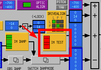
- Abilitate the IM TEST channels for longitudinal, pitch and yaw. In the example below those channels they are off.
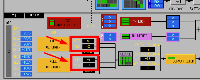
Align the oplev beam to the centre of the QPDs. Use the IM test channels to move the marionette such that the readout of the oplev in Normalized Displacement Units (ndu) are close to zero. In ndu the displacement varies within [ -100 , 100 ] ndu with linear range approximately [ -50 , 50 ] ndu.
Use diaggui to open the file SRM_TM_OPLEV_L_PREDIAG.xml, carry out the measurement and save the results.
Use diaggui to open the file SRM_TM_OPLEV_P_PREDIAG.xml, carry out the measurement and save the results.
Use diaggui to open the file SRM_TM_OPLEV_Y_PREDIAG.xml, carry out the measurement and save the results.
Open the file SRM_TM_OPLEV_L_PREDIAG.xml again. At the TM-L resonant frequency around 0.656 Hz. (Actuation along y_len.)
Take a note of the amplitudes x_len and y_len in the plot "ADS: x_len (red), y_len (blue)" using the cursor feature of diaggui.
Because the actuation is along TM-L, which is associated to y_len, set y_len > 0 as a convention.
Take a note of the relative phase between x_len and y_len in the plot "Transfer function: x_len and y_len relative phase".
If the phase is around 0° set x_len > 0.
If the phase is around ±180° set x_len < 0.
Take note of the amplitudes x_tilt and y_tilt in the plot "ADS: x_tilt (red), y_tilt (blue)".
Take note of the relative phase between y_len and x_tilt using the red line in the plot "Transfer function: x_tilt (red), y_tilt (blue) phase, additional information".
If the phase is around 0° set x_tilt > 0.
If the phase is around ±180° set x_tilt < 0.
Take note of the relative phase between y_len and y_tilt using the blue line in the plot "Transfer function: x_tilt (red), y_tilt (blue) phase, additional information".
If the phase is around 0° set y_tilt > 0.
If the phase is around ±180° set y_tilt < 0.
Open the file SRM_TM_OPLEV_P_PREDIAG.xml. At the TM-P resonant frequency around 0.820 Hz. (Actuation along y_tilt.)
Take note of the amplitudes x_tilt and y_tilt in the plot "ADS: x_tilt (red), y_tilt (blue)".
Because the actuation is along TM-P, which is associated to y_tilt, set y_tilt > 0 as a convention.
Take note of the relative phase between x_tilt and y_tilt; use the plot "Transfer function: x_tilt and y_tilt relative phase".
If the phase is around 0° set x_tilt > 0.
If the phase is around ±180° set x_tilt < 0.
Take note of the amplitudes x_len and y_len in the plot "ADS: x_len (red), y_len (blue)" using the cursor feature.
Take note of the relative phase between y_tilt and x_len using the red line in the plot "Transfer function: x_len (red) and y_len (blue) phase, additional information".
If the phase is around 0° set x_len > 0.
If the phase is around ±180° set x_len < 0.
Take note of the relative phase between y_tilt and y_len using the blue line in the plot "Transfer function: x_len (red) and y_len (blue) phase, additional information".
If the phase is around 0° set y_len > 0.
If the phase is around ±180° set y_len < 0.
Open the file SRM_TM_OPLEV_Y_PREDIAG.xml. At the TM-Y resonant frequency around 1 Hz. (Actuation along x_tilt.)
Take a note of the amplitudes x_tilt and y_tilt in the plot "ADS: x_tilt (red), y_tilt (blue)".
Because the actuation is along TM-Y, which is associated to x_tilt, set x_tilt > 0 as a convention.
Take note of the relative phase between x_tilt and y_tilt; use the plot "Transfer function: x_tilt and y_tilt relative phase".
If the phase is around 0° set y_tilt > 0.
If the phase is around ±180° set y_tilt < 0.
Take note of the amplitudes x_len and y_len in the plot "ADS: x_len (red), y_len (blue)" using the cursor feature.
Take note of the relative phase between x_tilt and x_len using the red line in the plot "Transfer function: x_len (red) and y_len (blue) phase, additional information".
If the phase is around 0° set x_len > 0.
If the phase is around ±180° set x_len < 0.
Take note of the relative phase between x_tilt and y_len using the blue line in the plot "Transfer function: x_len (red) and y_len (blue) phase, additional information".
If the phase is around 0° set y_len > 0.
If the phase is around ±180° set y_len < 0.
Open the Matlab file oplev_diagonalization_script.m.
- Scroll down to around line 109 and make sure the right-hand side of the five listed assignments refer to the suspension you are working with (BS, SR2, SR3, SRM). The example shown here corresponds to SR2.
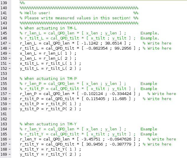
- Scroll down to around line 140 and write the information in the section according to the examples, which are commented lines.
- Save the script and execute it.
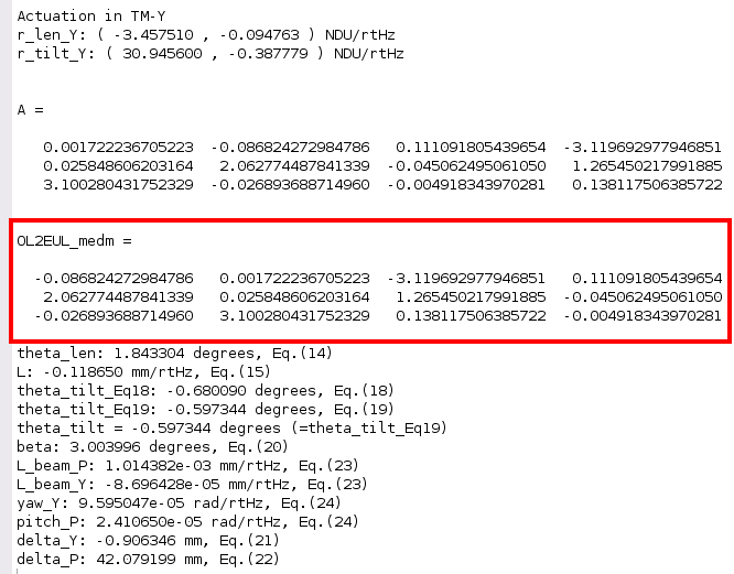
The output of the script includes is a matrix called OL2EUL_medm. Copy this matrix into the medm screen.
 .
. 
Run diagnosis. Item yet to be written.
Write a klog with the following format (preferably). Item yet to be written.


